Tutorial: running and analyzing a simulation
This page will walk you through running a simulation and analyzing the output, in the process discussing many of the key features of HallThruster.jl. An interactive Jupyter notebook tutorial covering similar topics and convering the process of comparing the results of the code to an established benchmark is also available here.
Defining geometry
The first thing we need to simulate a Hall thruster is geometry. Let's invent a fictional Hall thruster with a channel length of 3 cm, inner channel radius of 5 cm, and outer channel radius of 6.5 cm. To define the geometry, we create a HallThruster.Geometry1D object:
using HallThruster

# All units are in meters!
my_geometry = HallThruster.Geometry1D(
    inner_radius = 0.05,
    outer_radius = 0.065,
    channel_length = 0.03
)
For clarity and ease of readability, you may also input dimensional numbers from the lovely Unitful package as shown below:
using HallThruster
using Unitful

# Units will be correctly converted!
my_geometry = HallThruster.Geometry1D(
    inner_radius = 5.0u"cm",
    outer_radius = 6.5u"cm",
    channel_length = 3.0u"cm"
)
Magnetic field
The next thing we need is a magnetic field function. This can by any callable object, so long as it takes in an axial location in meters and returns a magnetic field strength in Teslas. Let's use a magnetic field with a Gaussian shape and a peak radial magnetic field strength of 200 Gauss at the channel exit plane:
function my_magnetic_field(z)
    if z < 0.03
        return 0.02 * exp(-((z - 0.03) / 0.02)^2)
    else
        return 0.02 * exp(-((z - 0.03) / 0.04)^2)
    end
end
Alternatively, we may want to load in a magnetic field from a file. Suppose we have a magnetic field stored in a file my_bfield.csv which has the following first few lines:
z(m),Br(T)
0.0,0.0021079844912372868
0.001,0.0024430133907998
0.002,0.0028171684184209005
0.003,0.0032324238493067863
0.004,0.003690390479859787
0.005,0.004192227743021959
0.006,0.004738555173642436
0.007,0.005329365956270483
0.008,0.005963945588597749
0.009,0.006640798906893217
0.01,0.00735758882342885
...
We could load this in using the DelimitedFiles package
my_magnetic_field_data, header = readdlm("my_bfield.csv", ',', header=true)We can then construct a function which interpolates the data (here a linear interpolation, but you can use more complex interpolations using the Interpolations.jl package):
z_data = my_magnetic_field_data[:, 1]
Br_data = my_magnetic_field_data[:, 2]
my_magnetic_field_itp = HallThruster.LinearInterpolation(z_data, Br_data)
Creating a Thruster
Once we have a geometry and a magnetic field, we can construct a Thruster:
my_thruster = HallThruster.Thruster(
	name = "My thruster",
    magnetic_field = my_magnetic_field,
    geometry = my_geometry,
    shielded = false,
)
In addition to a magnetic field and a geometry, we have also provided a name (optional) and designated whether the thruster is magnetically shielded or not. If true, then the electron temperature used for electron wall loss computations will be the anode temperature instead of the temperature on centerline. HallThruster.jl also includes a built-in definition for the widely-known SPT-100 thruster, accessible as HallThruster.SPT_100.
Defining a Config
We can now define a Config. We will run a simulation using Xenon propellant and two ion charge states, with a discharge voltage of 300 V and a mass flow rate of 6 mg/s. For anomalous transport, we use a multi-zone Bohm-like transport model. Many more options than these can be tweaked. For more information and a list all possible options, see the Configuration page.
my_config = HallThruster.Config(
    ncharge = 2,
    discharge_voltage = 300u"V",
    thruster = my_thruster,
    domain = (0.0u"cm", 8.0u"cm"),
    anode_mass_flow_rate = 8.0u"mg/s",
    wall_loss_model = HallThruster.WallSheath(HallThruster.BoronNitride),
    anom_model = HallThruster.MultiLogBohm([0.02, 0.03, 0.04, 0.06, 0.006, 0.2]),
    propellant = Xenon,
    neutral_velocity = 500.0u"m/s",
    neutral_temperature = 500.0u"K",
    ion_temperature = 500.0u"K",
    cathode_Te = 2.5u"eV",
    anode_Te = 2.5u"eV",
    ion_wall_losses = true,
)
Running a simulation
Now we can run a simulation. To do this, we use the run_simulation function. In addition to the Config object we just created, we also pass in the grid we want to run the simulation with, the number of frames we want to save, the timestep, in seconds and the simulation duration (also in seconds).
julia> @time my_solution = HallThruster.run_simulation(my_config; grid= EvenGrid(150), nsave=10000, dt=1e-8, duration=1e-3)
 36.058672 seconds (783.66 k allocations: 519.964 MiB)
Hall thruster solution with 10000 saved frames
Retcode: success
End time: 0.001 seconds
Postprocessing and analysis
Once you have run a Hall thruster simulation, you will want to analyze the results to see how your simulation performed. This section describes the utilities available for such tasks.
The Solution object
Running a simulation returns a HallThruster.Solution object, which has the following fields:
t: A vector of times at which the simulation state is saved u: A vector of simulation state matrices saved at each of the times in t savevals: A Vector of NamedTuples containing saved derived plasma properties at each of the times in t retcode: A Symbol describing how the simulation finished. This should be :Success if the simulation succeeded, but may be :NaNDetected if the simulation failed. params: A NamedTuple containing simulation parameters, such as the Config the simulation was run with, the computational grid, and more. params.cache contains all of the variables not contained in u
Extracting performance metrics
After running a simulation, the two things we might care the most about are the predicted thrust and discharge current. These can be computed with the thrust and discharge_current functions, respectively.
julia> HallThruster.thrust(my_solution) # Thrust in Newtons at every saved frame
10000-element Vector{Float64}:
 0.24759825170838257
 0.23553180163085566
 ⋮
 0.1677545384599781
 0.1677545384591017

julia> HallThruster.thrust(my_solution, 12) # Thrust in Newtons at the twelfth frame
0.16887856098607704
julia> HallThruster.discharge_current(my_solution) # Discharge current in A at every frame
10000-element Vector{Float64}:
16.594260447976414
16.491449186956455
⋮
12.635410795570154
12.63541079552306
julia> HallThruster.discharge_current(my_solution, 1999) # Discharge current in A at the 1999th frame
12.137864749597252
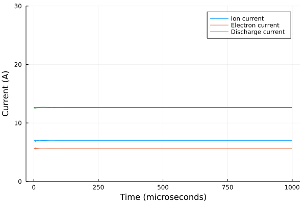
We can plot the ion, electron, and total currents using our plotting package of choice. In this case, we use Plots
using Plots
time_us = my_solution.t .* 1_000_000 # Convert time from seconds to microseconds
I_ion = ion_current(my_solution)
I_total = discharge_current(my_solution)
I_electron = I_total .- I_ion # we can also just type electron_current(my_solution)

p = plot(
    time_us, I_ion;
    label = "Ion current",
    xlabel = "Time (microseconds)",
	ylabel = "Current (A)"
)
plot!(p, time_us, I_electron; label = "Electron current")
plot!(p, time_us, I_total; label = "Discharge current", linewidth = 2)

display(p)
Time averaging results
In the above case, the simulation settled to a steady state after 250 microseconds, so we could just look at the last frame to obtain our performance and plasma properties. However, Hall thrusters are often oscillatory. To see this, let's cut the minimum anomalous collision frequency in half and re-run the simulation. The new config is:
my_config = HallThruster.Config(
    ncharge = 2,
    discharge_voltage = 300u"V",
    thruster = my_thruster,
    domain = (0.0u"cm", 8.0u"cm"),
    anode_mass_flow_rate = 8u"mg/s",
    wall_loss_model = HallThruster.WallSheath(HallThruster.BoronNitride),
    # change second to last number here from 0.006 to 0.003
    anom_model = HallThruster.MultiLogBohm([0.02, 0.03, 0.04, 0.06, 0.003, 0.2]),
    propellant = Xenon,
    neutral_velocity = 500.0u"m/s",
    neutral_temperature = 500.0u"K",
    ion_temperature = 500.0u"K",
    cathode_Te = 2.5u"eV",
    anode_Te = 2.5u"eV",
    ion_wall_losses = true,
)
Plotting the current, we find that the solution now no longer converges to a steady value but instead oscillates strongly about a mean:
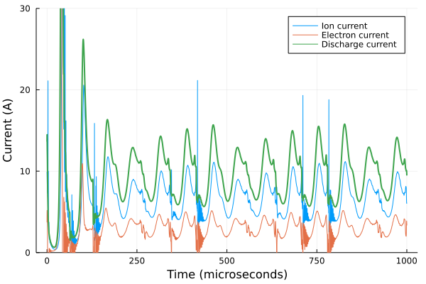
To compute performance, we want to average over several of the oscillations. To do this, we employ the time_average function
julia> my_time_average = time_average(my_solution)
Hall thruster solution with 1 saved frames
Retcode: Success
End time: 0.001 seconds
The time_average function returns another Solution object, just like my_solution, with a single saved frame holding the time-averaged simulation data. In the case of our oscillatory simulation above, the simulation doesn't settle into a stationary mode until about 100 microseconds have elapsed (about 1000 frames, since we saved 10000 total). If we want to only average the last 9000 frames, we would type
julia> my_time_average = time_average(my_solution, 1000) # start averaging at frame 1000Plotting
HallThruster.jl includes plotting recipes to allow you to plot your simulation results if the Plots package is installed. To plot the last frame of the simulation, you can type:
using Plots

plot(my_solution)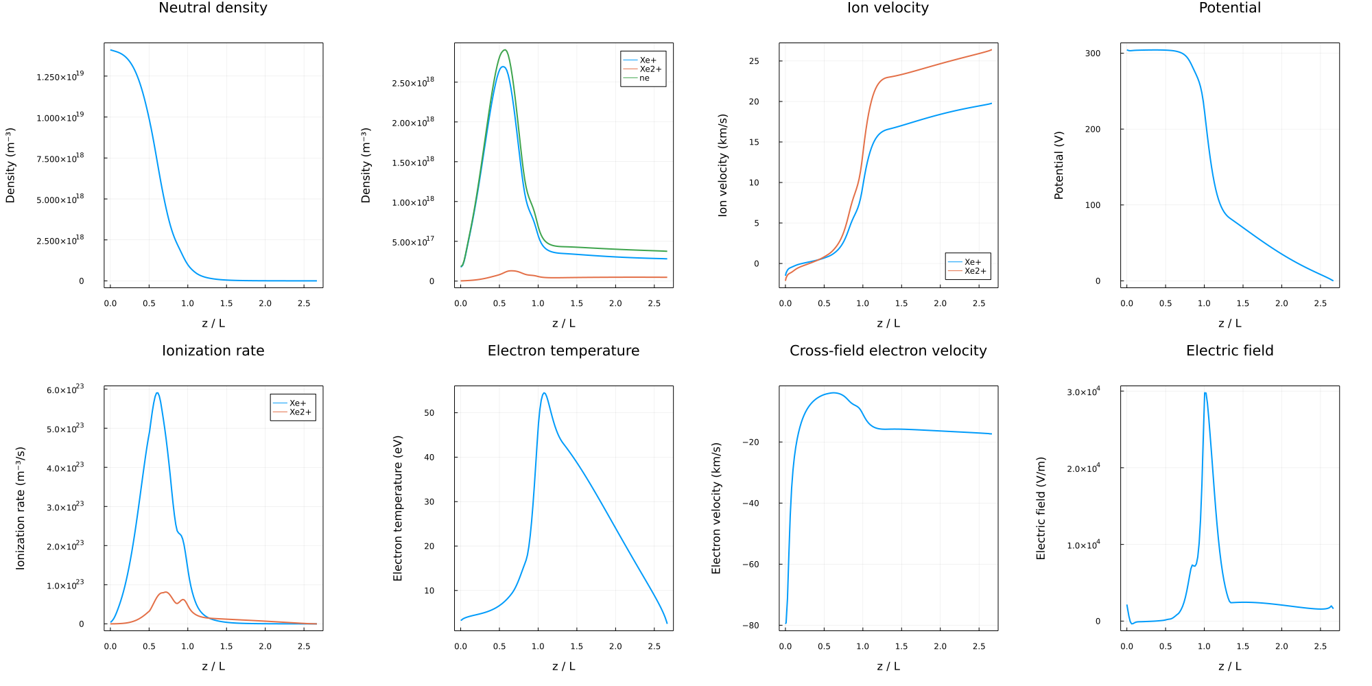
To plot a different frame, you can do plot(my_solution, frame_you_want). You can also plot time averaged solutions, as they are no different from a standard solution. You can also plot certain parts on a log scale using the yaxis=:log argument, add labels using label = "label", and plot solutions over each other using plot!, just as normal using Plots.jl.
Computing efficiencies
There are several key efficiency metrics that are employed to judge how well a Hall thruster performs. The most common is the anode efficiency, defined as the ratio of thrust power to power put into the plasma:
\[\eta_a = \frac{1}{2}\frac{T^2}{\dot{m} V_d I_d}\]
We can compute this using the compute_anode_eff function, which returns the anode efficiency at every timestep:
julia> HallThruster.anode_eff(my_solution)
10000-element Vector{Float64}:
 0.769654845938557
 0.7008079984180736
 ⋮
 0.46399997114634145
0.46399997114322283When computing time-averaged efficiencies, it is better to first time-average the simulation and then compute the efficiencies from the averaged plasma properties then it is to average the instantaneous efficiencies. For example,
avg_eff = mean(HallThruster.anode_eff(my_solution))  # not ideal
avg_eff = HallThruster.anode_eff(time_average(my_solution)[] # better
The mass utilization efficiency is the ratio of the ion beam mass flow rate to the total anode input mass flow rate and is computed with compute_mass_eff:
julia> HallThruster.mass_eff(my_solution)
10000-element Vector{Float64}:
 1.3406882897286088
 1.2966376960524595
 ⋮
 1.0022667540786294
 1.0022667540739632
The current utilization efficiency is the ratio of the ion current to the discharge current:
julia> HallThruster.current_eff(my_solution)
10000-element Vector{Float64}:
 0.599052550532874
 0.58182111692138
 ⋮
 0.552664262832069
 0.5526642628312223
The voltage utilization efficiency is the ratio of the effective acceleration voltage to the discharge voltage:
julia> HallThruster.voltage_eff(my_solution)
10000-element Vector{Float64}:
 0.9962185160007747
 0.9699301625865606
 ⋮
 0.8856545575551746
 0.8856545575546175
Extracting plasma properties
To access a plasma property, you index the solution by the symbol corresponding to that property. For example, to get the plasma density at every frame, I would type:
julia> ne = my_solution[:ne]
10000-element Vector{Vector{Float64}}:
...
This returns a Vector of Vectors containing the number density at every frame and every cell. To get the number density just in the 325th frame, I would type
julia> ne_end = my_solution[:ne][325]
152-element Vector{Float64}:
 9.638776090165182e16
 9.638776090165182e16
 1.1364174787296864e17
 ⋮
 2.568578735293536e17
 2.532630941584664e17
 2.532630941584664e17
This has 152 elements, one for each of the 150 interior cells and 2 for the left and right boundary. To get the axial locations of these cells in meters, we can access sol.params.z_cell.
For ion parameters (ion density and velocity), we specify which charge state we want to extract. For example, to get the velocity (in m/s) of doubly-charged Xenon at the 4900th frame, we would type:
julia> ui = my_solution[:ui, 2][4900]
152-element Vector{Float64}:
 -1795.4362688519843
 -1724.298256534735
 -1647.858433966283
     ⋮
 27654.42396859592
 27735.77112807524
 27735.756446024698
Here, indexing by [:ui, 2] means we want the velocity for doubly-charged ions. We could similarly index by [:ni, 1] for the density of singly-charged ions.
A list of parameters that support this sort of indexing can be found by calling HallThruster.saved_fields(). A few of these are:
B: Magnetic field strength in Teslaωce: Cyclotron frequency in Hzνan: Anomalous collision frequency in Hzνe: Total electron collision frequency in Hzνc: Classical collision frequency in Hzνei: Electron-ion collision frequency in Hzνen: Electron-neutral collision frequency in Hzνex: Excitation collision frequency in Hzνiz: Ionization collision frequency in Hzradial_loss_frequency: Electron-wall collision frequency for wall loss calculation in Hzνew_momentum: Electron-wall collision frequency for mobility calculation in Hzμ: Electron mobilityE: Electric fieldϕ: plasma potential at cell centers in VTev: Electron temperature in eVpe: Electron pressure in eV/m^3∇pe: Electron pressure gradientnn: Neutral densityni: Ion density (default 1st charge state, index by[:ni, Z]to get charge stateZ)ui: Ion velocity (default 1st charge state, index by[:ui, Z]to get charge stateZ)
Saving simulations for use as restarts
To save a simulation for later, you can use the write_restart function. We can then read it back with the read_restart function:
julia> HallThruster.write_restart("my_restart.jld2", my_solution);
julia> HallThruster.read_restart("my_restart.jld2")
Hall thruster solution with 10000 saved frames
Retcode: Success
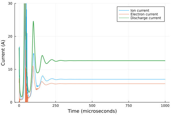
End time: 0.001 secondsTo use a restart as the initial condition for a simulation, you can use the restart keyword argument in the run_simulation function:
julia> @time my_solution = HallThruster.run_simulation(my_config; ncells=150, nsave=10000, dt=1e-8, duration=1e-3, restart = "my_restart.jld2")
 34.700016 seconds (7.27 M allocations: 1016.374 MiB, 0.79% gc time, 5.42% compilation time)
Hall thruster solution with 10000 saved frames
Retcode: Success
End time: 0.001 seconds
If we plot the currents, we see that the simulation remained at the steady state established in the initial run: